Model Confusion Matrix
Building a model is just the beginning of the deep-learning journey. After you create a deep-learning model, you want to know how effective it is—how well it solves the problem that you identified when you began.
Evaluating the effectiveness of a model involves analyzing the model metrics. The terminology and concepts behind model metrics can be confusing at first, so we’ll try to demystify these concepts by using your actual data and real-world examples. Then you can apply these techniques to better understand your own Einstein Vision or Language model.
The confusion matrix shows you how well each label (also called a class) in your model performs. You can use this information to evaluate whether you need to add more data to a label or add a different type of data to a label.
When you train a model, the training process randomly selects and holds out some of the data. After the model is created, the training process validates the model by sending the holdout data for prediction. This validation process creates the confusion matrix values.
It can be difficult to interpret the confusion matrix and understand what to do with the information that it provides These steps walk you through the entire process and assume no prior knowledge.
The first step is to get the model metrics data for your model and build the confusion matrix from that data. The model metrics and confusion matrix data returned by the API vary based on the model type. This process covers the confusion matrix for models with a modelType of:
- text-intent
- text-sentiment
To build the confusion matrix for your model, you make an API call to get the metrics.
-
Identify the correct model metrics endpoint.
Einstein Language GET
https://api.einstein.ai/v2/language/models/<MODEL_ID>The response from this call differs based on the type of dataset that the model was created from:text-intentortext-sentiment. However, the model metrics for a language model always contains alabelsarray and aconfusionMatrixarray. -
Replace
<MODEL_ID>with the ID of your model, and use cURL or Postman to make the API call.
The cURL call to get the model metrics looks like this.
The call to get the model metrics returns a response similar to this JSON.
Now that you have the model metrics data for your model, you use that data to build the confusion matrix. As you step through this process, you build the matrix manually. But you use the same logic to create the array programmatically.
- When you look at the
labelsarray in the response JSON, you see two labels in this model. Add one to the number of labels and then create a table with that number of columns and rows. In this case, the table has three rows and three columns.
- Enter each value in the labels array in the column and row headers in the same order that the labels appear in the array. Your matrix now looks like this table.
| Mountains | Beaches | |
|---|---|---|
| Mountains | ||
| Beaches |
- Look at the
confusionMatrixarray in the JSON response. It contains an array of numbers for each label. The arrays match the order of the labels: the first array contains predictions for the examples labeled Mountains, and the second array has predictions for the examples labeled Beaches. Add these numbers to the matrix.
| Mountains | Beaches | |
|---|---|---|
| Mountains | 5 | 2 |
| Beaches | 0 | 5 |
Now your confusion matrix is complete!
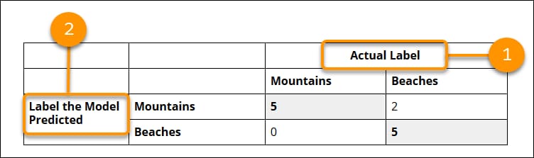
To make the confusion matrix easier to read, one trick is to add a row to the top with the heading Actual Label and a column to the left with heading Label the Model Predicted. After you get more familiar with the confusion matrix, you might not need to add the extra labels.
- Across the top, are the actual labels (Mountains, Beaches) of the validation examples from your dataset.
- On the left side, are the labels (Mountains, Beaches) that the model predicted for those examples.
Of the 12 examples that were held out for validation and have the actual label Mountains, the model predicted that:
- 5 are in the label Mountains
- 0 are in the label Beaches
Of the six examples that were held out for validation and have the actual label Beaches, the model predicted that:
- 5 are in the label Beaches
- 2 are in the label Mountains
The bold numbers in the matrix indicate the correct predictions. The correct predictions are always positioned in the diagonal cells of the table, which makes it easier to read.
| Mountains | Beaches | |
|---|---|---|
| Mountains | 5 | 2 |
| Beaches | 0 | 5 |
The confusion matrix gives you a visual explanation of your model’s accuracy. For the test data, it shows you how many examples it predicted correctly and incorrectly and which label it predicted the examples were in.
This confusion matrix is based on a small dataset. But you can still see that the model was confused about two images: It predicted that two examples labeled Beaches belong in the Mountains class.
The model gave incorrect predictions for two examples that are labeled Beaches. This is quite a high percentage (about 40%), given that this is a small dataset. Now what can you do with this information? Here are some guidelines on how to use the confusion matrix and possible issues that it identifies.
The model is created from your labeled data, so the first thing to do is to go back to your data. With a small dataset, an easy step to take is to manually scan the data in the labels that the model is confusing. Check whether any patterns emerge from the source data or how it’s labeled. Sometimes data is added with the wrong label, which you can fix by relabeling the data and creating a new dataset and model.
The model metrics don’t tell you which examples were held out for validation and which of those examples were misclassified. After you create a model, you can programmatically identify the misclassified images by taking all the images from the dataset that you used to create the model and sending them in for a prediction. You call one of these endpoints depending on the model type.
- image:
/predict - text-intent:
/intent - text-sentiment:
/sentiment
After you identify the misclassified images, you can analyze them to see what the issue might be. Were the images mislabeled before they were added to the dataset? In the beaches and mountains scenario, do the misclassified images contain both a beach and a mountain? If so, you could consider removing the misclassified images from your dataset.
On the other hand, if you think images that are similar to the misclassified images will come in for prediction—for example, images with both beaches and mountains—consider adding a new label and corresponding examples to your dataset and model.
When the confusion matrix reports misclassification, try adding more data to the misclassified labels. The beach-mountain dataset has only two labels, so you could add more data to both labels and then re-evaluate the confusion matrix.
When you train a dataset to create a model, the training process holds out a percentage of the data for validating the model and uses the rest to create the model. The ratio of test data versus training data is called the split ratio.
When you call the /train endpoint, the training process test data percentage defaults to 10 percent for vision models and 20 percent for language models. You can also specify this ratio by using the trainSplitRatio parameter.
To get more information about test data and training data, use the API call to get the training status. The call looks like this cURL command.
From the following response, you can see:
- 99 examples (images) in total
- 87 examples used to train the dataset and create the model
- 12 examples held out to validate the model
Going back the confusion matrix, if you total up all the numbers in the matrix, that number is equal to the testSplitSize—the number of examples held out to test the model.
Now let’s look at an example from a model with more labels. You can create this Einstein Intent model by following the steps in Einstein Intent Quick Start.
The cURL call to get the model metrics looks like this.
The call to get the model metrics returns a response similar to this JSON. The precision recall curve data has been removed for brevity.
Follow the previous steps to create the confusion matrix. It looks like this table.
| Order Change | Sales Opportunity | Billing | Shipping | Password Help | |
|---|---|---|---|---|---|
| Order Change | 4 | 0 | 0 | 4 | 0 |
| Sales Opportunity | 0 | 7 | 0 | 1 | 0 |
| Billing | 0 | 0 | 2 | 0 | 0 |
| Shipping Info | 1 | 1 | 0 | 7 | 0 |
| Password Help | 0 | 0 | 0 | 0 | 4 |
This confusion matrix points to a few areas in the data that you might want to investigate. First, if you look at the Shipping Info column, you see that the model is misclassifying a large percentage of text labeled “Shipping Info.” In particular, the model is classifying quite of few of those examples (4 out of 12) as “Order Change.”
For this case, it would be helpful to send all the examples used to create the dataset into the model for prediction to identify which examples were misclassified. Then you can use that information to identify patterns in the data or labeling that requires correction.
When you train an intent dataset and use the multilingual-intent-ood algorithm, the model handles text that doesn't fit into any one of the model labels. Text that doesn't fit into any of the model labels is also called out-of-domain (OOD) text.
There are some differences in the model metrics and learning curve data for an OOD model.
- The f1 score and all other metrics are returned only for the model labels.
- The confusion matrix includes numbers for the labels in the model as well as for the OOD label. However, the
labelsarray includes only labels in the model. It doesn't include an OOD label.
Building the confusion matrix for an OOD model requires one extra step. When you build the confusion matrix for an OOD model, you must manually add a label to the labels array. You can name the label any value. Then when you loop through the numbers in the confusionMatrix, the last number in each array, and the last array itself, is associated with the OOD label.
For example, the labels array for a case routing OOD model might look like this JSON.
The confusionMatrix array returns six arrays and each array has six elements. "confusionMatrix":[[4,1,0,0,1,2],[0,7,0,0,0,0],[3,0,2,0,1,2],[0,0,0,2,1,1],[1,0,0,0,1,1],[0,0,0,0,0,0]]
When you build the confusion matrix, be sure to add a sixth label to the labels array so that the matrix is correct: Shipping Info, Sales Opportunity, Order Change, Password Help, Billing, Out of Domain. The final confusion matrix using this data looks like this table.
| Shipping Info | Sales Opportunity | Order Change | Password Help | Billing | OOD | |
|---|---|---|---|---|---|---|
| Shipping Info | 4 | 1 | 0 | 0 | 1 | 1 |
| Sales Opportunity | 0 | 7 | 0 | 0 | 0 | 0 |
| Order Change | 3 | 0 | 2 | 0 | 1 | 1 |
| Password Help | 0 | 0 | 0 | 2 | 1 | 1 |
| Billing | 1 | 0 | 0 | 0 | 1 | 1 |
| OOD | 0 | 0 | 0 | 0 | 0 | 0 |