timeseries

Uses existing data to predict future data points. The timeseries statement must follow a projection statement in your query. Perform any filtering pre-projection or after the timeseries statement.

timeseries crunches your data and selects the forecasting model that gives the best fit. You can let timeseries select the best model or specify the model you want. timeseries detects seasonality in your data. It considers periodic cycles when predicting what your data will look like in the future. You can specify the type of seasonality or let timeseries choose the best fit.

The amount of data required to make a prediction depends on how your data is filtered and grouped. For example, for a non-seasonal monthly model, 2 data points are sufficient, whereas for a seasonal monthly model, at least 24 data points (two seasonal cycles) are required. If you don’t have enough data to make a good prediction, timeseries returns nulls in the data. If no data is passed to timeseries, an empty dataset is returned.

1result = timeseries resultSet generate (measure1 as fmeasure1 [, measure2 as fmeasure2...]) with (parameters);

measure1, measure2, and so on, are the measures that you want to predict future values for. You can predict measures from grouping queries or from simple values queries. The predicted values and the original values are projected together. The columns from the previous foreach statement are also projected.

parameters can have the following values:

• length (required) Number of points to predict. For example, if length is 6 and the dateCols type string is Y-M, timeseries predicts data for 6 months.

  If you want to use dateCols but your data stream has missing dates, use fill before using timeseries.

  timeseries makes the most accurate prediction possible by choosing the best algorithm for your data. Predictive algorithms are more accurate for shorter time periods.

  Note

• dateCols (optional) Date fields to use for grouping the data, plus the date column type string. For example, dateCols=(CloseDate_Year, CloseDate_Month, "Y-M"). Date columns are projected automatically. Allowed values are:

  • YearField, MonthField, "Y-M"
  • YearField, QuarterField, "Y-Q"
  • YearField, "Y"
  • YearField, MonthField, DayField "Y-M-D"
  • YearField, WeekField "Y-W"

• ignoreLast (optional) If true, timeseries doesn’t use the last time period in the calculations. The default is false.

  Set this parameter to true to improve the accuracy of the forecast if the last time period contains incomplete data. For example, if you’re partway through the quarter, timeseries forecasts more accurately if you set this parameter to true.

• order (optional) Specify the field to use for ordering the data. Mandatory if dateCols isn’t used. By default, this field is sorted in ascending order. Use desc to specify descending order, for example order=('Type' desc). You can also order by multiple fields, for example order=('Type' desc, 'Group' asc).

  For example, suppose that your data has no date columns, but it has a measure column called Week. Use order='Week'.

  Specify either dateCols or order.

  Note

• partition (optional) Specify the column used to partition the data. The column must be a dimension. The timeseries calculation is done separately for each partition to ensure that each partition uses the most accurate algorithm. For example, data in one partition can have a seasonal variation while data in another partition doesn’t. The partition columns are projected automatically.

  For example, suppose that your sales data for raw materials contains the date sold, type of raw material, and the weight sold. To predict the future weight sold for each type of raw material, use partition='Type'.

• predictionInterval (optional) Specify the uncertainty, or confidence interval, to display at each point. Allowed values are 80 and 95. The upper and lower bounds of the confidence interval are projected in columns named column_name_low_95 and column_name_high_95.

• model (optional) Specify which prediction model to use. If unspecified, timeseries calculates the prediction for each model and selects the best model using Bayesian information criterion (BIC).

  Allowed values are:

  • None timeseries selects the best algorithm for the data
  • Additive uses Holt’s Linear Trend or Holt-Winters method with additive components.
  • Multiplicative uses Holt’s Linear Trend or Holt-Winters method with multiplicative components

• seasonality (optional) Use with dateCols to specify the seasonality for your prediction. Allowed values are:

  • 0 No seasonality
  • any integer between 2 and 24

  If unspecified, timeseries calculates the prediction for each type of seasonality and selects the results with the smallest error.

  Example

  seasonality	dateCols	Type of Seasonality
  seasonality=4	dateCols="Y-Q"	Yearly seasonality, because there are four quarters in a year.
  seasonality=12	dateCols="Y-M"	Yearly seasonality, because there are 12 months in a year.
  seasonality=7	dateCols="Y-M-D"	Weekly seasonality, because there are seven days in a week.

Here’s how you can make the most of using timeseries:

• Are you currently part way through the month, quarter, or year? Consider setting ignoreLast to true so that timeseries doesn’t use the partial data in the current time period, leading to a more accurate prediction.
• Is timeseries not returning any data? If there aren’t enough data points to make a good prediction, timeseries returns null. Try increasing the number of data points.
• Is timeseries returning an error? You could have gaps in your dates or times. Like all good forecasting algorithms, timeseries needs a continuous set of dates with no gaps, including in each partition. If you think your data has date gaps, try using fill first.

Suppose that you run a chain of retail stores, and the number of tourists in your city affect your sales. Use timeseries to predict how many tourists will come to your city next year:

1q = load "TouristData";
2q = group q by ('Visit_Year', 'Visit_Month');
3q = foreach q generate 'Visit_Year', 'Visit_Month', sum('NumTourist') as 'sum_NumTourist';
4
5-- If your data is missing some dates, use fill() before using timeseries()
6-- Make sure that the dateCols parameter in fill() matches the dateCols parameter in timerseries()
7q = fill q by (dateCols=('Visit_Year','Visit_Month', "Y-M"));
8
9-- Use timeseries() to predict the number of tourists.
10q = timeseries q generate 'sum_NumTourist' as Tourists with (length=12, dateCols=('Visit_Year','Visit_Month', "Y-M"));
11
12q = foreach q generate 'Visit_Year' + "~~~" + 'Visit_Month' as 'Visit_Year~~~Visit_Month', Tourists;

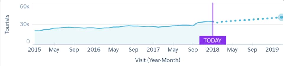
Use a timeline chart and set a predictive line to see the calculated future data. The resulting graph shows the likely number of tourists in the future.

Suppose that you wanted to predict the number of tourists in your city next year with 95% accuracy. Use predictionInterval=95 to set a 95% confidence interval for the number of tourists. The upper and lower bounds are projected as the fields Tourists_high_95 and Tourists_low_95.

1q = load "TouristData";
2q = group q by ('Visit_Year', 'Visit_Month');
3q = foreach q generate 'Visit_Year', 'Visit_Month', sum('NumTourist') as 'sum_NumTourist';
4
5-- If your data is missing some dates, use fill() before using timeseries()
6-- Make sure that the dateCols parameter in fill() matches the dateCols parameter in timerseries()
7q = fill q by (dateCols=('Visit_Year','Visit_Month', "Y-M"));
8
9-- use timeseries() to predict the number of tourists
10q = timeseries q generate 'sum_NumTourist' as 'fTourists' with (length=12, predictionInterval=95, dateCols=('Visit_Year','Visit_Month', "Y-M"));
11q = foreach q generate 'Visit_Year' + "~~~" + 'Visit_Month' as 'Visit_Year~~~Visit_Month', coalesce(sum_NumTourist,fTourists) as 'Tourists', fTourists_high_95, fTourists_low_95;

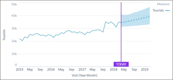
Use a timeline chart and set a predictive line to see the calculated future data. In the timeline chart options, select Single Axis for the Axis Mode, fTourists_high_95 for Measure 1, and fTourists_low_95 for Measure 2. The resulting graph shows the likely number of tourists in the future and the 95% confidence interval.

Suppose that you want to predict the revenue for each type of account. You know that your account revenue has yearly seasonality and that you want to group dates by quarter, so you specify dateCols=('Date_Sold_Year','Date_Sold_Quarter', "Y-Q") and seasonality = 4. To see the predicted values over the next year, use length=4 to specify four quarters.

1q = load "Account";
2q = group q by ('Date_Sold_Year', 'Date_Sold_Quarter', 'Type');
3q = foreach q generate 'Date_Sold_Year', 'Date_Sold_Quarter', 'Type', sum('Amount') as 'sum_Amount';
4
5-- If your data is missing some dates, use fill() before using timeseries()
6-- Make sure that the dateCols parameter in fill() matches the dateCols parameter in timerseries()
7q = fill q by (dateCols=('Date_Sold_Year','Date_Sold_Quarter', "Y-Q"), partition='Type');
8
9-- use timeseries() to predict the amount sold
10q = timeseries q generate 'sum_Amount' as Amount with (partition='Type',length=4, dateCols=('Date_Sold_Year','Date_Sold_Quarter', "Y-Q"), seasonality = 4);
11q = foreach q generate 'Date_Sold_Year' + "~~~" + 'Date_Sold_Quarter' as 'Date_Sold_Year~~~Date_Sold_Quarter','Type', Amount ;

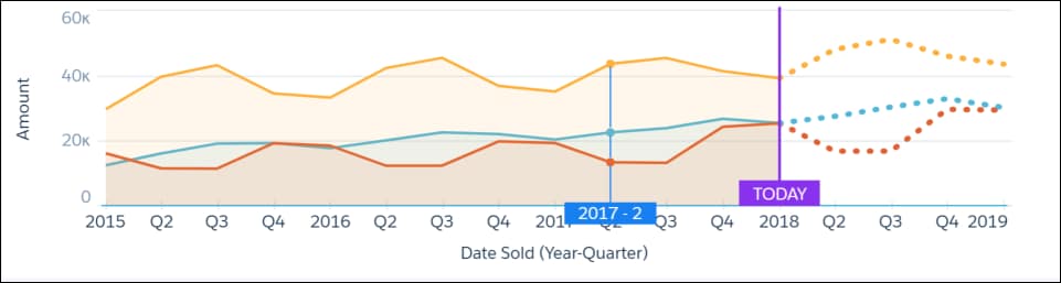
Use a timeline chart and set a predictive line to see the calculated future data. The resulting graph shows the likely sum of revenue for each account, taking into account the quarterly seasonal variation.

See Also

• Forecast Future Data Points with timeseries
• arimax

j

Overview

Quick Start

Examples

SAQL Reference

SAQL Basic Elements

SAQL Operators

SAQL Statements

arimax

cogroup

fill

filter

foreach

group-by

group-by rollup

join semi and anti

limit

load

offset

order

sample

timeseries

union

SAQL Functions

Query Performance

Previous Versions